I’ve been having a preliminary flick through Andrew Gelman’s book, (amazon) which so far seems excellent. I thought I’d have a shot at the questions in the introductory chapter.
First question. Easy, no problem.
Second question. Ooh, bit trickier. Got there in the end.
Third question. This has taken me 40 minutes, which seems like justification for posting a solution on this ‘ere weblog.
so the question is asked:
Suppose that in each individual in a population there is a pair of genes, each of which can be either X or x, that controls eye colour: those with xx have blue eyes, those with XX or Xx or xX have brown eyes. Those with Xx are known as heterozygotes.
The proportion of individuals with blue eyes (xx) is  , and the proportion of heterozygotes is
  .
.
Each parent transmits one gene to the child: if the parent is a heterozygote, the probability that they transmit X is  . Assuming random mating, show that amongst brown eyed parents with brown eyed children, the proportion of heterozygotes is
  .
.
Okay says I, it’s just Bayes’ rule, no? Let’s denote all heterozygotes as Xx (this should save significant keypresses…), children as ch and parents as pa.
Under Bayes rule we need a likelihood 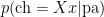 , prior
  and a ‘marginal likelihood’ term, which we get by summing the above. So we’re going to get something like:

We also need to make sure that we only consider brown eyed individuals (XX, Xx, and xX. not xx). let’s have a look at the priors:


and a little manipulation yeilds:
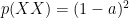
So looking at combinations of parents who have brown eyes:


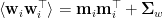
Each of which can be considered a prior, with correspondings likelihoods (of the child being Xx):


Now, the top line of Thomas Bayes’ famous rule looks like:

remembering that the bottom line must consist of all brown eyed children of brown eyed parents (not just the heterozygotes), the bottom line looks like:

Phew. Cancelling a few terms does indeed leave

Not going to school for years switches your brain off: It took me as long to figure out how to do this as it did to blog it…
There’s actually a second part to the problem, (first set by Lindley, 1965, apparently), which turns out to have some rather messy terms in. I think I’ll save blogging that for another day.


.